Chapter 9 ~ Personal Finances
⬆ Shiftrefresh Shift-Refresh this page to see the most up-to-date instructions.
Search the word adulting and you'll find many articles and videos about how to manage your money. Many college students do not yet track how much they earn and how much they spend and in what categories. Sure, your bank statements or online accounts may show you what you've deposited and spent, however, if your bank doesn't show you a combined total for income and spending categories, then you may be clueless as to where you're overspending, which reduces your chances to save for emergencies or important purchases (like a vacation!).
Creating your own balance statement in a spreadsheet will enable you to see how you're fairing, financially. In this chapter, you'll start by creating your own template for capturing monthly income and expenses for the year, then average the totals and subtract expenses from income to see what the discretionary amount is. That discretionary amount will help you with Chapter 10's assignment.
If you are married with or without children, then consider including their income and expenses in your sheet.
If you've done this before, then it'll be quick work. If you haven't, then block out a couple of hours at the start, then throughout the week, add more details as you find them.
This chapter's skills and discussion will take between 4 and 12 hours to complete.
Print these instructions.
The following procedure has many steps, which are perhaps easier to follow when you print and check them off as you go. Hide/close + the previous section to avoid printing too many pages.
9.1 Design a Personal Finance Sheet.
In this lesson, you'll design a simple spreadsheet to document the current year's income and expenses. The year-to-date income and expenses will be added and averaged to provide a quick overview of your financial situation. This work is not a budget; it is a description of your current state of financial affairs.
Use real amounts whenever possible but don't add account names or numbers. No one else will see your data but the Instructor and TAs. Keep the information generic for the assignment, then when the term is over, add more detail to suit your needs, so you can use it as a template year after year. We don't download your file but it is archived in Canvas. If you are concerned about using your own real data, then you can use the data provided in the screenshots below.
Still concerned? Reach out to the instructor for guidance.
Do count expenses paid by family members as income...you'll see how in step 9.3.
- Launch a spreadsheet application:
- Microsoft Excel. Recommended for Business and Science-related majors. Save the file often with Ctrls or ⌘s.
- Google Sheets. Recommended for inexperienced students who are not Business majors.
- Apple Numbers. Not all of the required tasks are possible using this application. No technical support will be provided.
Abigail Hill demonstrates how to set up the personal finance sheet in Google Sheets on MacOS. (2022) Khalid Aljohani demonstrates how to set up the personal finance sheet in Google Sheets on Windows in Arabic. (2022) - Open a Blank worksheet file and save the filename as Personal Finances First and Last name. Move the file to your CS 101 folder.
- Name the worksheet 202_ Income Expenses (for the current year) by double-clicking the untitled tab at the bottom.

- Type or copy/paste the following list of categories into Column A.
Select all rows and columns then set the font to Tahoma or Lato:

Income
Job/wages
Family support
Financial aid
From savings accounts
Total income

Expenses
Tuition and fees
Books and materials
Rent or mortgage
Water & sewer
Electric power
Gas/propane/oil (heating)
Garbage service
Phone service
TV and internet service
Groceries, dining, drinks
Clothing
Household items
Car loan
Gas and oil changes
Car insurance
Entertainment
Personal care
Pets
Medical care
To savings accounts
Other loan payments
Credit cards payments
Total expenses

Total discretionary
Don't leave any of these row headings out. If you don't have those expenses, you'll give them a 0 zero amount later.
Also, it is OK to leave the text and background colors because they are subtle. You may change them if you like, but be sure the background color is subtle... no bright colors allowed because they can reduce readability and increase eye fatigue. - Click on the Row 1 selector on the left. Apply Bold using Cntlb or ⌘b.
Do the same for these rows: Total Income, Expenses, Total Expenses
and Total Discretionary.
Bold the entire row, not just the heading.
Once you add data later, you may need to apply bold to the row again.

- Label Column B with Monthly Average.

- Add January to column C1,
then drag the cell to the right to auto-fill (magic!) the remaining months of the year (eleven columns).

- Freeze, Wrap, and Resize columns and rows:
- Select the row of headings and View > Freeze it (so it will show even when scrolling down to the bottom of the sheet.)
- Stretch column A to the right so that all of the longer row headings don't spill into the next column.
- Reduce the width of the remaining columns so they are not wider than necessary.
- Stretch row 7 Expenses down a bit so it creates space between it and the Total Income heading.
- Do the same for the Total Discretionary row.
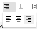
- Shift-click on all of the columns A through N.
Then, click the align right button.
- Shift-click on columns B through N and
apply the Currency number format, so that all numbers are displayed as dollars.
Feel free, however, to use your own country's monetary symbol instead,
so you can to apply your country's amounts, rather than American amounts.
- Microsoft Excel
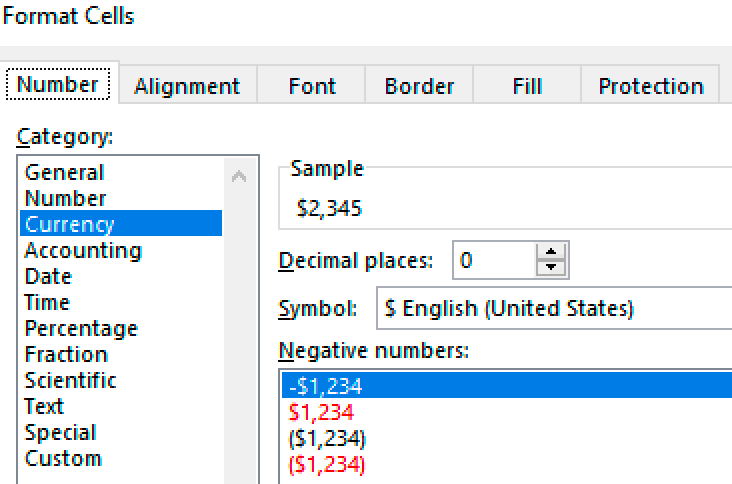
or
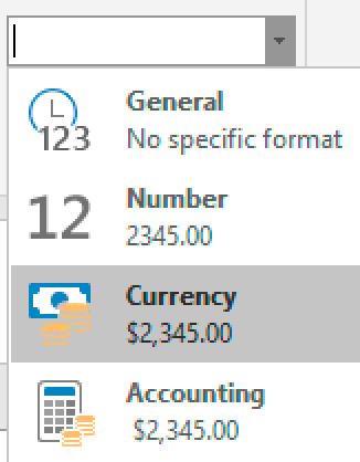
- Google Sheets
$ or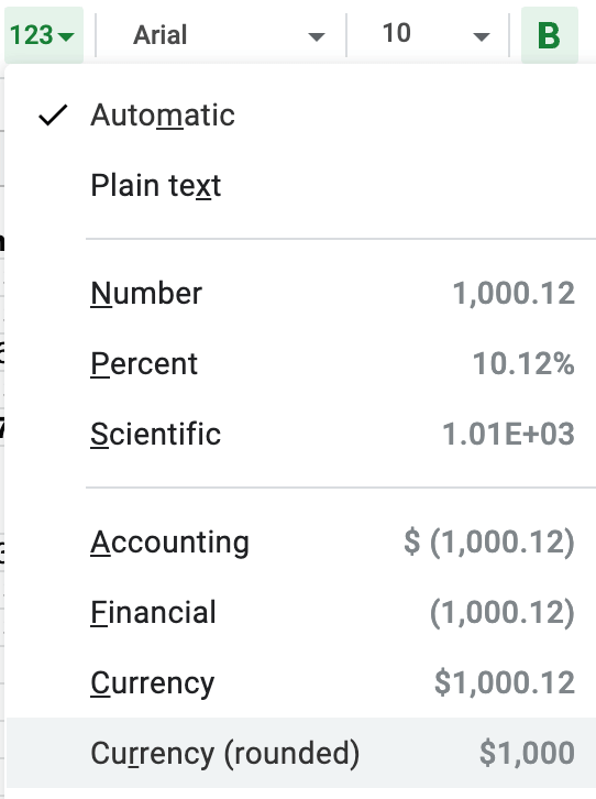
- Microsoft Excel
- Type 1000 in the C2 cell, so you can see what the numbers look like.
And, reselect columns B through N then
choose the .0 ← or .0 → icon to remove the decimal places.
Even if you typed dollars and cents using a decimal, this button will remove the cents so you display only whole numbers.
 Only whole numbers will be allowed for this assignment, which improves readability...you want to analyze at a glance what you've got available.
9.2 Add and calculate income data.
Add the average function to column B so that all income amounts are averaged. Add actual amounts in columns C to N to correlate with column A's Income categories.
- To see the average of all 12 months' income source totals,
add the =AVERAGE() function to cell B2
then between the parenthesis, include the range of cells C2:N2.

Delete the formula from the Expenses/Monthly Average cell B7; it won't have any data to process.
- Before you begin to enter more data, remember:
- This sheet is not a budget; it is an actual accounting.
- When a monthly income amount is exactly the same from month to month,
drag its cell handle to the right to automatically fill in the same amount for each month of the year.

- Don't however, add amounts to future months if you don't know those amounts yet, as you cannot predict the future.

- From your monthly pay stubs, if any, locate the income for each month of the year (so far) and add them to the monthly cells
in the Jobs/Wages row of your sheet.
If you get paid weekly or bi-weekly instead of monthly, then click into the cell and use math to add two or more paycheck amounts together, like this:
=400+200. The final number in the cell will be 600.
If you can't locate your pay stubs and your online banking app doesn't show those deposits, but know your hourly rate of pay,
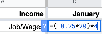
then calculate an estimated pay amount. For example: $10.25 per hour for 20 hours per week for 4 weeks can be calculated like this:
=(10.25*20)*4.
- For the Family row, add a 0 zero if family doesn't provide help with any expenses. If they do help with expenses, then wait until you add those expense amounts in step 9.3. All expenses paid for by family will be totaled as income once you have that data entered.
- For the Financial aid row, you may have received a lump sum at the start of each term.
Add those amounts to the months you received them. and 0 for the months you did not.
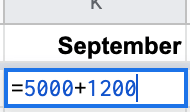
If you have aid from various sources, use math in the cell to add them together, for example:
- For the From savings accounts row, enter the amounts you took out of savings accounts each month to pay for expenses. We'll consider that income for this lesson.
- To get the total income for each month, start by
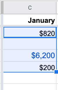
selecting the number cells in column C2 to C5 (January's incomes),
then, choose the ∑SUM
option to auto-fill the sum of numbers in the B6 Total Income cell.
A typical formula looks like this: sum(C2:C5), which means you want the total of numbers in column C rows 2 through 5.
 →
→
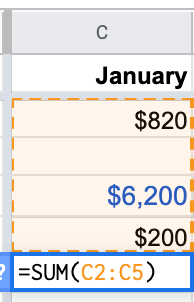
Finally, drag January's total income cell C6 to the right to auto-fill through to December.
9.3 Add and calculate expense data.
For each item in Column A's Expenses section, add an actual amount spent in columns C to N for each month.
Use math in cells where multiple amounts were spent.
Leave future months blank unless those future amounts are the same as previous months.
When a monthly expense amount is exactly the same from month to month (for example, the rent or mortgage),
drag its January amount to auto-fill the remaining months.

- For the Tuition and fees cells, type the amount of tuition paid at the start of each term or the monthly amount. Don't enter months you don't pay tuition. If someone else pays your tuition, reflect the amount here then see step 9.3.24 about how to count it as income.
- For the Books and materials cells, use math to sum each term's books and materials expenses.
- For the Rent or mortgage cells, add your portion of monthly amount paid for your dorm, apartment, or house.
Include renter's insurance, home owner's insurance, and property taxes as needed.
If you live with family who pays your portion of the rent or mortgage, then ask them for the total mortgage expense
and divide it by the number of people who live in the house. Use math in that cell to calculate it.
For example, if two parents and a sibling live in the family home, then a mortgage of $1720 per month divided by 4 people is:
=1720/4. Your portion of the rent/mortgage is $430.

Unless you were homeless or camped in a free zone, your portion of the rent for the dwelling where you slept must be provided up to the current month. - For the Water and sewer cells, find the amount on your water bill if you live alone. Otherwise, use math to calculate your portion of the monthly amount if roommates are involved or family pays it. If you live in the dorm or apartment where this expense is part of your rent payment, just add a 0 amount.
- For the Electric power cells, find the amount on your electric bill if you live alone. Otherwise, use math to calculate your portion of the monthly amount if roommates are involved or family pays it. If you live in the dorm or apartment where this expense is part of your rent payment, just add a 0 amount.
- For the Gas/propane/oil heating cells, find the amount on your heating bills if you live alone. Otherwise, use math to calculate your portion of the monthly amount if roommates are involved or family pays it. If you live in the dorm or apartment where this expense is part of your rent payment, just add a 0 amount.
- For the Garbage service cells, find the amount on your garbage bills if you live alone. Otherwise, use math to calculate your portion of the monthly amount if roommates are involved or family pays it. If you live in the dorm or apartment where this expense is part of your rent payment, just add a 0 amount.
- For the Phone service cells, find the amount on your landline/cellphone bill(s) if you live alone. Otherwise, use math to calculate your portion of the monthly amount if roommates are involved or family pays it. If you have a monthly rental and data amount, itemized on a family bill, use math calculate your portion, or locate it in the online account.
- For the TV and internet service cells, find the amount on your monthly invoices if you live alone. Otherwise, use math to calculate your portion of the monthly amount if roommates are involved or family pays it.
- For the Groceries, dining, and drinks cells, use math to add up the total of receipts for a month's expenses for food, restaurants, and coffee, tea, and alcohol. If you don't save paper receipts, then look for the amounts at the checking account and/or credit card registers in your online bank account.
- For the Clothing cells, find the amount on your clothing receipts. Use math to calculate the total of purchases for each month when you bought clothes.
- For the Household items cells, find the amount on your household items receipts. Use math to calculate the total of purchases for each month when you bought them. Household items include furniture, appliances, decor, and gardening supplies.
- For the Car loan cells, enter the amount of your car payments (even if someone else pays it). If you don't own a car, enter 0 zero for each month.
- For the Car gas and oil changes cells, use math to enter the amount of receipts for a month's worth of gas and oil changes (even if someone else pays for them). If you don't own a car, enter 0 zero for each month.
- For the Car insurance cells, enter the monthly amount or the lump sum if you pay quarterly or biannually (even if someone else pays it). If you don't own a car, enter 0 zero for each month.
- For the Entertainment cells, use math to add up expenses for activities like online streaming services, cinema/movie/theatre, concerts, museums, club dues, cover charges, etc.
- For the Personal care cells, enter the typical cost of haircuts, nail care, and other grooming for the months you had them. If you don't get your hair/nails done professionally, enter a 0 zero for each month.
- For the Pets cells, use math to enter expenses such as food, vet bills, and accessories. If you don't have a pet, enter a 0 zero for each month.
- For the Medical care cells, use math to enter expenses such as medications, office visits, and equipment rental/purchases. Enter a 0 zero for each month you did not have medical expenses.
- For the Savings account cells, enter the amount you added to savings accounts, if any. If you don't save yet, enter a 0 zero for each month.
- For the Other loans cells, enter amounts of loan payment(s) you made. If you have more than one, use math in the cells to add up the monthly payments. If you don't have other loans, enter a 0 zero for each month.
- For the Credit cards cells, enter the amounts paid each month to reduce the balance due. If you have more than one, use math in the cells to add up the monthly payments. If you don't use credit cards, enter a 0 zero under each month.
- To create the Total for expenses,
select the number cells in column C (January), cells 8 through 25,
then choose the ∑SUM option to auto-fill the sum of numbers in the
Total Expense cell.
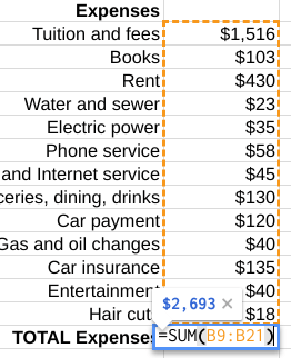
Drag the new January Total Expenses cell to the right to autofill the remaining months' totals.
-
Complete the Family Income cell:
For all of the expenses that someone else paid, combine them by using math and selections. For example, if your parents paid your cellphone and car insurance bills, then click into the Family Income cell for January and type =. Then, while that cell is still selected, click on the C13 cell, then type a +, then click into the C18 cell. Click Enter. Data from the two cells gets added to the Family cell as income. Drag the new January total cell to the right to autofill the remaining months' totals for family income.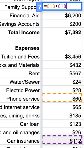
Using this method will allow you to keep an accurate sum for those items, so you understand what it really costs to live.
9.4 Determine discretionary funds.
The discretionary amount is the difference between income and expenses...it is typically what is left over in a checking account.
- Determine how much you have left over by clicking into the Discretionary Funds cell for January.
Type =,
click the C column's Total Income cell,
then type the - minus/hyphen key,
then click the C column's Total Expenses cell.
This will subtract the Total Expenses from the Total Income.
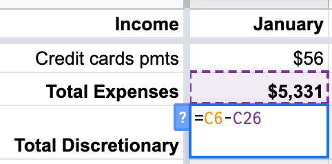
Drag the cell to the right to auto-fill the remaining months' discretionary amounts. - If your discretionary amount is positive,
then you theoretically have some leftover money to move into a savings account
to be used for emergencies and fulfilling dreams.

- If your discretionary amount is negative,
then you spent more than you earned.
This could be because some of the monthly amounts are incorrect or missing.
Or, it could be you're using a credit card to pay for expenses.
Or, you used the previous months' discretionary amounts in addition to the current month's remaining in checking.

- Make corrections to the amounts, so they are more accurate. The goal is to account for everything you earn and spend, so the discretionary amount should be near zero $0 or a small positive amount. If you had negative amounts, did your checking account reserves (previous months' discretionary amounts) help expend that amount, or did you pull from Savings? If you pulled from Savings, then be sure to account for it in the Income area.
- Select all Total rows, then apply the Bold style. Those row headings as well as the data will be easier to read if each is bold.
9.5 Print the sheet.
In this step, you'll be printing your sheet as a single PDF file. Use the skills you learned in the previous chapter to output with these specifications:
- Narrow margins (to allow more room for the columns).
- Fit-to-page (so the entire sheet fits on one page).
- Landscape orientation (horizontal).
- File name (which includes your name) displayed in the header at the top left.
- Current date displayed in the header at the top right.
9.6 Ask for help.
Stuck on a specific step? Share your file with the instructor.
In order for the instructor and TAs to see your progress without having to download or ask for account permission, provide a correctly-set sharing URL so they can look at it live. Follow the most appropriate instructions below.
Paste the sharing URL into the Canvas Inbox message or Assignment Comment box, along with your questions. Note which step number you're stuck on.
Share Microsoft Office files from the OSU OneDrive cloud drive and share Google Suite files from the OSU Google cloud drive:
- Windows or Microsoft Account
- Login to your OSU OneDrive account from the browser.
- Drag the file from your hard drive to the OSU OneDrive file list in the browser to transfer it there.
- Beside the file name in the list, click the
 Share icon:
- Choose the settings provided in the screenshot below:
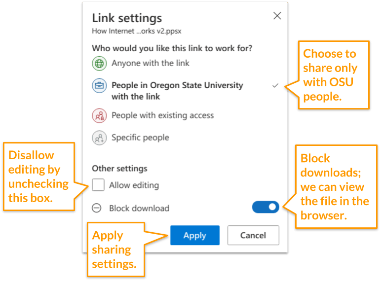
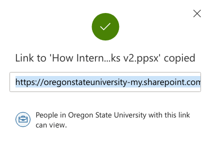
- Copy the link so you can provide it to the instructor or in the Assignment Comment box.

- Google Account
- With your file open, click the Sharing button at the top right of the screen. Or, if the file is not open but listed in the Drive, right-click it to choose the Share menu.
- Click the Get Link box to update the OSU Settings and copy the link:

- Ignore the Share with People and Groups box for this course.

Paste the URL into the Canvas Inbox message or Assignment Comment box, along with your questions. Note which step number you're stuck on.
9.7 Verify your work.
Doesn't your new document look great!
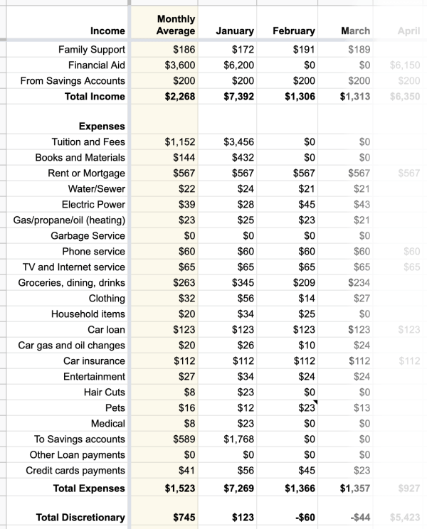
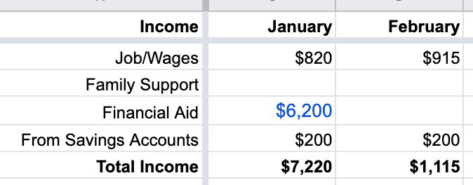
← The results of your worksheet should look something like the screenshot at the left.
Notice that all numbers are whole (no decimals) and aligned to the right. Number columns are always aligned to the right in spreadsheets. The row headings also align to the right to improve readability. Space is provided between Income totals and Expenses to make it easy to differentiate them. All Total rows and column headings are bold. Optional subtle background colors are allowed on columns and total rows.
After the course is over, continue to use this spreadsheet every month of every year to see what you're taking in and spending, then it'll be easier to plan for the future. Add a new sheet with the next year as the name, and copy over the categories in column A to help you get started. Customize the headings of the next year's sheet to help you track specific accounts. Also copy over any data that stays the same throughout the year. Be sure to back it up to an additional secure drive.
From the Canvas Home tab, click the Ch 9 ~ Personal Finances assignment. Scroll to the bottom to see the Rubric. Compare your work to the Rubric to ensure you've included all paragraphs and design elements as well as reviewed/edited your work. The rubric is based on the following scoring criteria, which are based on the instructions above: Check off each criterion to confirm you've completed them before submitting the file.
- Sheet is free of plagiarism.
- Sheet is printed as PDF with narrow margins, fit-to-page in landscape orientation, and filename/student name and date displayed in the header.
- Sheet includes all required income and expenses categories in the first column.
- Sheet includes reasonably accurate data in all 12 months of the current year in columns.
- Sheet includes Sum totals for 12 months of income and expenses.
- Sheet includes Discretionary totals for all 12 months.
- Sheet uses the Average function in column B to show an average of all 12 months per category.
- Column headings and Total rows are bold.
- Numbers render as right-aligned whole numbers with dollar signs (no decimal places).
9.8 Submit the file.
Each assignment must be submitted before the Due date and time as specified on the Canvas Home tab. The Available Until date and time constitutes a grace period, which can be used in an emergency, or if you are ill (it cannot be used for every assignment). Students who submit using the Available Until date may incur score reduction. Students on a DAS Flexibility Contract: there is no need to notify the instructor. All of your Available Until dates will be set to 72 hours past the Due Date, which can be used up to 3 times. Abuse of the Flexibility Contract will be reported to DAS.
- Click on the Canvas Home button and scroll down to the Ch 9 ~ Personal Finances assignment. Click the assignment link.
- Upload the PDF file. Confirm that it uploaded.
- Within 3 days of submission, be on the lookout for Rubric feedback and Comments from the TA and Instructor.
- Ask questions about the score and feedback in the assignment's Commenting box.
